The code is open-source and available on Github.
Discussion on Hacker News
As a first blog post, I decided to describe a way to detect first stories (a.k.a new events) on Twitter as they happen. This work is part of the Thesis I wrote last year for my MSc in Computer Science in the University of Edinburgh.You can find the document here.
Every day, thousands of posts share information about news, events, automatic updates (weather, songs) and personal information. The information published can be retrieved and analyzed in a news detection approach. The immediate spread of events on Twitter combined with the large number of Twitter users prove it suitable for first stories extraction. Towards this direction, this project deals with a distributed real-time first story detection (FSD) using Twitter on top of Storm. Specifically, I try to identify the first document in a stream of documents, which discusses about a specific event. Let’s have a look into the implementation of the methods used.
Implementation Summary
Upon a new tweet arrival, the tweet text is split into words and represented into the vector space. It is then compared with the N tweets it is most likely to be similar to, using a method called Locality Sensitive Hashing. This data clustering method dramatically reduces the number of comparisons the tweet will need to find the N nearest neighbors and will be explained in detail later below. Having computed the distances with all near neighbor candidates, the tweet with the closest distance is assigned as the nearest. If the distance is above a certain threshold, the new tweet is considered a first story. A detailed version of the summary above will follow in the description of the bolts which act as the logical units of the application.
Why Storm?
If Storm is new to you, Storm is a distributed real-time computation system which can guarantee data processing, high fault-tolerance and horizontal scaling to significantly large amounts of input data. It simplifies the implementation of parallel tasks by providing a programming interface suitable for stream processing and continuous computation. Having such a volume of input tweets streamed in real-time, FSD seemed like an ideal use case for Storm framework which can scale up the work by adding more resources.

Topology – network of spouts and bolts
Each application must define a network of spouts and bolts before it starts running. This network is called a topology and contains the whole application logic. Spouts are the entry point of the system and are responsible for reading data from external sources such as the Twitter streaming API. Bolts on the other hand are the logical units of the application and can perform operations such as running functions, filtering, streaming aggregations, streaming joins and updating databases.
How it works
Upon a new tweet arrival, the short text is split into words so that a partial counting can be applied. In an attempt to reduce the lexical variation that occurs in different documents, a small normalization set of out-of-vocabulary (OOV) words has been used. Words like “coz” are replaced with “because” and “sureeeeeeeeeeeeeee” with “sure”. Porter Stemming algorithm was considered as an extra step here but was not applied as it didn’t improve the accuracy of the final results. Having replaced the OOV words, the URLs and mentions (@) are removed from the tweet text.
The algorithm continues by representing each tweet in the vector space using the TF-IDF (Term Frequency – Inverted Document Frequency) weighting. By applying the weighting, words that appear more frequently are expected to have lower weight in contrast to the rarer ones. Each vector is also normalized using the Euclidean norm. Given a term 


is the total number of documents that the term t appears in.
Having converted the tweet to vector, we will apply the Locality Sensitive Hashing (LSH) algorithm to find the nearest neighbor candidates. LSH method aims to benefit from a reduced number of comparisons required to find the approximate (1 + ε)-near neighbors among a number of documents.
The idea behind it is to use hash-tables called buckets for similar points (tweets). According to this approach, whenever a new point (tweet) arrives, its hash value will be computed and it will be stored into several buckets. Inside the same bucket, the probability of collision with similar documents is much higher. In other words, tweets that have an identical hash with the arriving tweet are nearest neighbor candidates. By using this method, we will not compare a “weather” tweet with a “music” one as most probably they are not related. I should remind you that we need to find the tweet with the shortest distance to the arriving tweet. The figure below helps to understand the core LSH mechanism by showing what happens in each bucket.
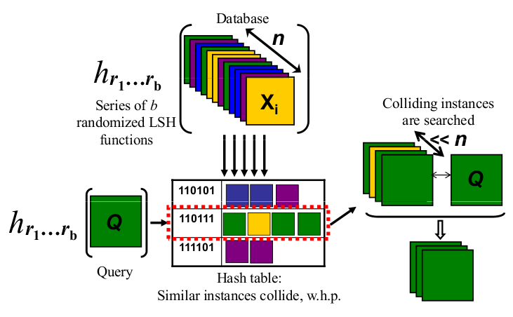
Locality sensitive hashing logic
By increasing the number of buckets used you repeat the process of hashing to find more nearest neighbors. Therefore more comparisons are made and the probability to find a closer neighbor is increased. Different buckets give different hashes for the same tweet, as the hash value is created using the random projection method. According to this, k random vectors are assigned to each bucket. Each random vector consists of values derived from a Gaussian distribution N(0, 1). Τhe binary hash value consists of k bits each of which is calculated using the below function.

where r is the random vector and u the tweet vector. Each hash bit is a Dot Product. The concatenation of all hash bits will form the hash which will be stored inside each bucket. At this example, 13 bits were used to define the length of the hash. The less bits you use, the more collisions you will find, thus more comparisons to make. However, the effort to compute the dot product for each bucket would be reduced. Limitation: Storing tweets into all buckets would require infinite memory for the hashing of all previously seen tweets. To prevent this from happening, we keep up to 20 tweets with the same hash per bucket.
The interesting part in applying the LSH algorithm lies in the hash property. The fact that incoming tweets will be compared with only the tweets that have the same hash, as opposed to all previously seen ones is the beauty of it. It greatly reduces the comparisons required to find the closest neighbour.
Having gathered the nearest neighbors from all buckets we compare the distance between the tweet and the nearest neighbors using the cosine similarity measure. The cosine similarity between two vectors 

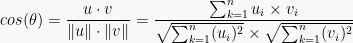
As an extra step, the tweet is also compared to a fixed number of most recently seen tweets. The neighbor with the shortest distance (the highest cosine score) is assigned as the nearest and the distance represents the score of the tweet. If a tweet has score above a certain threshold, it is identified as a First Story.
Code Explained…
** If you don’t have any previous experience with Storm I highly recommend this tutorial to learn the basic elements such as functions, grouping, aggregations and familiarize yourself with the streaming logic. The codebase depends heavily on them. However the logic is the same and can be implemented outside Storm too. **
Now the above procedure would benefit from the scalability and the parallelism Storm can offer. Different steps of the algorithm can be split into bolts and achieve faster results when running on a cluster. Luckily, Storm offers a local cluster mode which simulates a cluster.
All input tweets have been gathered using Twitter4J and a crawler class. Tweets are mostly in English and written one per line in a text file as JSON. Having gathered a significant number of tweets, let’s feed them into the system.
The tweets are emitted one by one into the topology. I’m using a Storm built-in mechanism (called DRPC) to request the result for a tweet. The DRPC allows an application to parallelize an intense function on top of Storm and call that function from within your application to get the results back. Hence the Distributed Remote Procedure Call. The following code is located in the main method. It emits the data into the topology and saves the results to a file. Note that the input stream can equally be a real-time feed instead of a file, such as a Twitter spout implementation reading off the Twitter API.
while ((tweetJson = br.readLine()) != null) {
   String result = drpc.execute(TOPOLOGY_NAME, tweetJson);
   fos.write(result.getBytes());
   fos.write(newLine);
}
The topology design is explained in separate steps below.
TridentTopology topology = new TridentTopology();
topology.newDRPCStream(TOPOLOGY_NAME, drpc)
.each(new Fields("args"), new TextProcessor(), new Fields("textProcessed"))
.each(new Fields("textProcessed"), new VectorBuilder(),
   new Fields("tweet_obj", "uniqWordsIncrease"))
First, a TridentTopology object is created. The input argument in the TextProcessor function is the tweet object. TextProcessor processes the text of the tweet and removes any links and mentions this may contain. It has been observed that URLs and mentions add linearity to the number of distinct words seen in the corpus. Storing and processing linear growing unigrams would be catastrophic and therefore they have to be removed. In addition to that, these features are Twitter specific, and this system should work with any stream of documents. The function emits a tweet object which is the input to VectorBuilder function.
The VectorBuilder is responsible for converting the tweet into vector space. Specifically, it computes the term frequencies, creates the vector using TF-IDF weighting and updates the inverse document frequencies for the words seen. The vectors are 1-d sparse matrices and were implemented using the CERN Colt software package. The vectors are also normalized using the Euclidean norm. Finally the function emits the tweet object which contains the tweet vector and the numbers of new words found.
.broadcast()
.stateQuery(bucketsDB, new Fields("tweet_obj", "uniqWordsIncrease"),
   new BucketsStateQuery(), new Fields("tw_id", "collidingTweetsList"))
   .parallelismHint(4)
As shown in the second code block, the tweet object along with the new words found are the inputs to the BucketsStateQuery. A State query is how Storm manages a state of an object. This state can be either internal to the topology (e.g. in-memory) or backed by an external storage such as Cassandra or HBase. The state consists of a list of Buckets and this Query Function is responsible for returning the colliding tweets from each bucket to be compared with the input tweet at a later stage.
A Bucket is actually a hash-table. Each bucket has a k number of random vectors each of which an 1-d dense matrix of size k. A concatenation of the dot products between the tweet and the random vectors produces a hash for each bucket. Based on the LSH logic, similar tweets have high probability to hash to the same value. Therefore, tweets with the same hash in each bucket are possible near neighbors. A list of near neighbors from all buckets is returned as a result. The function also updates the random vectors of each bucket prior to computing the hash. This is to take into account the new words seen in the input tweet, if any. As a last step, the tweet is inserted into all buckets, to be considered against future tweets.
Now the .parallelismHint(4) line sets the stateQuery to be executed by 4 executors which actually means 4 threads. To better understand how Storm parallelism works I highly recommend this article by Michael Noll. We want each thread to receive the data for each tweet and this is what .broadcast() method is used for. The total number of buckets we define is now split in 4 separate threads.
The following diagram represents the flow of the logic for Code Blocks 2 and 3

Flow Chart 1 – Click to enlarge
.each(new Fields("collidingTweetsList"), new ExpandList(),
   new Fields("coltweet_obj", "coltweetId"))
.groupBy(new Fields("tw_id", "coltweetId"))
.aggregate(new Fields("coltweetId", "tweet_obj", "coltweet_obj"),
   new CountAggKeep(), new Fields("count", "tweet_obj", "coltweet_obj"))
.groupBy(new Fields("tw_id"))
.aggregate(new Fields("count", "coltweetId", "tweet_obj", "coltweet_obj"),
   new FirstNAggregator(3*L, "count", true),
   new Fields("countAfter", "coltweetId", "tweet_obj", "coltweet_obj"))
We now have a list of colliding tweets and we need to select a subset of tweets to be compared with the tweet in question. It would be too expensive in terms of computation to compare a tweet with all colliding ones. Note that the same tweet can be found as near neighbor from several buckets. Therefore, we perform a count on all identical tweets to find the ones that collide the most. Then we select the top 3*L to move forward for comparisons, where L the number of buckets.
In Storm, this is implemented using the Code Block 3. Since the output from BucketStateQuery is a list, the list returned is expanded to give a tuple that contains the colliding tweet object along with its id. This will help have a coltweetId per tuple and use the aggregate function of Storm. First we group by tweet_id to make sure we deal with tweets that collide only with this input tweet and we also group by colliding tweet ids to perform a count on them.
Then we use CountAggKeep which simply is a Count aggregator which keeps the input fields in the output. It must be noted here that the the aggregate operation removes any fields the tuple had before the aggregation except the grouping fields. This is opposed to the BaseFunction (e.g. each) that appends the output Fields at the end of the tuple. For this reason, I wrote a CountAggKeep aggregator that keeps the input fields in the output. As you may imagine, this only has meaning if the input fields have the same value in all tuples.
So far, the current computation gave us a tuple for each colliding tweet and a number of how many times this tweet was found in all buckets. We should then sort the tuples using a FirstNAggregator aggregator. This aggregator takes as input the max number of tuples to emit, the sorting field and the sorting order (true if reversed). “countAfter” is simply the “count” field, but renamed to meet the aggregator requirements. The aggregator requires that the output fields must correspond to the input fields and the sorting field not have the same name as before.
.each(new Fields("tw_id", "coltweetId", "tweet_obj", "coltweet_obj"),
   new ComputeDistance(), new Fields("cosSim"))
  .parallelismHint(2)
.shuffle()
.groupBy(new Fields("tw_id")) //sort to get the closest neighbour from buckets
.aggregate(new Fields("coltweetId", "tweet_obj", "coltweet_obj", "cosSim"),
   new FirstNAggregator(1, "cosSim", true),
   new Fields("coltweetId", "tweet_obj", "coltweet_obj", "cosSimBckts"))
We are now ready to make the comparisons between the tweet and the colliding tweets that exist in each tuple. ComputeDistance is the function which computes the cosine similarity between the tweets’ vectors and emits it as a value. Then a grouping by tweet id follows before sorting. FirstNAggregator is again used to sort the tweets on cosine similarity and only pick the closest colliding tweet to the input tweet.
This is a visual representation of the second logical part (Blocks 4,5).

Flow Chart 2 – Click to enlarge
.broadcast() //tweet should go to all partitions to parallelize the task
.stateQuery(recentTweetsDB, new Fields("tweet_obj", "cosSimBckts"),
   new RecentTweetsStateQuery(), new Fields("nnRecentTweet"))
   .parallelismHint(4)
.groupBy(new Fields("tw_id"))
.aggregate(new Fields("coltweetId", "tweet_obj", "coltweet_obj", "cosSimBckts"   , "nnRecentTweet"), new Decider(), new Fields("nn"))
.each(new Fields("nn"), new Extractor(),
   new Fields("colId", "col_txt", "cos"))
.project(new Fields("colId", "col_txt", "cos"));
Having found the closest tweet from buckets, the next step is to also compare the input tweet with a fixed number of most recently seen tweets. This is required only if the cosine similarity from buckets is low (compared to a given threshold). Otherwise, the tweet is not a first story anyway. RecentTweetsStateQuery is responsible for keeping a LinkedBlockingQueue<Tweet> queue of recently seen tweets. A parallelismHint of 4 is used to parallelize the task and each executor receives the tweet to make a comparison with its own queue. Note that the tweet is only stored in one of the 4 partitions each time, in a round robin fashion. The most recent tweet is appended in the end of the tuples.
Now there should be 4 tuples each of which containing the nearest neighbor from buckets and recent queue.
Then the Decider aggregator decides the result. The Decider is implemented using an aggregator of type Combiner. This partially aggregates the tuples (in each partition) before transferring them over the network to maximize efficiency, and might remind you how MapReduce uses combiners. According to the values in each tuple, it decides whether the closest tweet comes from the buckets or from the most recently seen tweets queue. Once found, it emits the NearNeighbour object which is the final closest tweet.
The object is processed by the Extractor function which extracts the information from the object and emits it as the final output. This is necessary as otherwise you would see the memory reference of the object as the result instead of the actual values. Since the tuple also contains the NearNeighbour object, we use the project operation of Storm to only keep the tuple fields we want in the result.
Example results
| Input tweet | Stored tweets | Similarity score |
| @Real_Liam_Payne i wanna be your female pal | i. wanna be your best friend so follow me 🙂 | 0.385 |
| RT @damnitstrue: Life is for living, not for stressing. | RT Life is for living, not for stressing. | 0.99 |
| East Timor quake leaves Darwin shaking: An earthquake off the coast of East Timor has be… http://t.co/UhfwCS2xPp | Everybody leaves eventually | 0.129 |
As we can see, the first row contains two tweets that are not so close to each other, hence the small similarity score. The second row contains a tweet and a retweet and therefore the similarity is very high. In the third row, the tweet is found to have a long distance from its nearest neighbor. This tweet can be identified as a first story. It is indeed talking about an 6.4-magnitude earthquake that took place in Darwin.
Note that to achieve reasonable results, a training period should first pass before start making decisions. This is required to let the buckets fill up with tweets and start producing accurate results. As time passes, less false alarms will occur.
But is a first story actually a first story?
It should be noted that an evaluation of the accuracy of this system (precision, recall) at such a scale would be impossible as it would require humans going through a very large number of tweets to manually label new events. However, an algorithm that detects new events with a similar implementation, has already been tested on newswire and broadcast news. It performs significantly well as shown in papers such as Petrovic et al., 2010.
Due to the limited text of tweets and the high volume of spam, the method should give a higher number of false alarms on Twitter. However, this can be restricted by creating topic threads on tweets. This means that a tweet should not be identified as first story unless a certain number of future tweets follow that speak of the same subject. This is a future improvement for this project and of course pull requests are welcome.
Performance on Storm
The same work has been carried on Storm 0.7.4 before Trident was out. I rewrote the codebase to benefit from the operations Trident can offer, such as grouping tuples on tweet id, sorting the tuples on cosine similarity, etc. The difference on Storm 0.8.2 was obvious both on performance and code elegance.
For the evaluation of this system a speedup metric was used. Specifically, I compared the performance of a distributed flavor of a first story detection system against a single/multi-threaded one. The parameters were set the same for both systems (e.g. number of buckets used, number of hash bits per tweet, etc.). The execution time refers to a dataset of 50K tweets on a 2-core machine setup. As shown below, Storm version clearly outperforms the single and multi-threaded versions.
| Speed-up (single-threaded) | Speed-up (multi-threaded) | |
| Storm | 1381 % | 372 % |
Final thoughts
The same approach can be used to group similar documents for different purposes such as near-duplicate detection, image similarity identification or even audio similarity.
As said in the beginning, the code is available on Github. I’d appreciate any code contributions / improvements and I wish you enjoyed the above long trip!

Great work. Twitter has just open sourced Summingbird, a streaming map reduce layer, that can run both on hadoop with Scalding and Stoem. Would be interesting how much code it saves you by implementing your code with it.
Nice blog post though.
Thanks, I heard about Summingbird. It looks cool.
[…] How to spot first stories on Twitter using Storm Source: https://micvog.com/2013/09/08/storm-first-story-detection/ 0 […]
[…] by jaapwalhout [link] […]
This might be of interest as well:
Click to access 1111.0352.pdf
As it turns out, there is an on-line variant of Bayesian non-parametrics k-means algorithm which is fairly similar in practice to what you do here.
For your initial text cleaning step you might want to try out https://github.com/brendano/ark-tweet-nlp/blob/master/src/cmu/arktweetnlp/Twokenize.java I’ve used it with good results.
This is an area of improvement for this project, thanks Ryan.
Isn’t a semantic analysis supposed to be more accurate than just hashing using random hashcodes? LSI/LSA perhaps – http://stackoverflow.com/questions/1746568/latent-semantic-indexing-in-java?
I suppose your question is to change the method (TF-IDF) for computing the tweet vector prior to applying LSH on it.
There is no such thing as LSH (random projection) vs LDA/LSI.
Now the hash’s random factor is minimized by applying the TF-IDF weighting prior to computing the hash, to provide a more accurate vector. Hence, words that appear more frequently such as “the” and “day” will have lower weight than “earthquake” and “rainbow”. One could use another method instead, such as LSI to identify patterns in the relationships between tweets. It would be interesting to make a comparison.
Btw consider using an ArrayDeque instead of ArrayList in the Bucket class. Remove(0) shifts all elements forward…wasteful.
ArrayDeque would perform better indeed. https://github.com/mvogiatzis/first-stories-twitter/issues/2
Hello,
Great article!
One question:
What do you use for OOV corrections ? Is there some open source toolkit for this?
Thank you,
Vlad Feigin
Thanks Vladi, I’m using words from a file. You can find it here: https://github.com/mvogiatzis/first-stories-twitter/blob/master/oov.txt . Any suggestions are welcome, this step could be more sophisticated.
[…] to whose scoop is the freshest, so to speak. Kobielus enunciates how he stumbled across 2013 blog: “How to spot first stories on Twitter using Storm”, wherein the Twitter user describes methods of detecting first stories “as they happen” using […]
Pretty nice post. I just stumbled upon your weblog and wished to say that I’ve truly enjoyed browsing your weblog posts.
In any case I’ll be subscribing on your feed and I’m hoping
you write again very soon!
I am doing nowadays a similar system to detect topics from twitter also, now I face a problem, that when I increase the parameter of number of permutations (L) I have many duplicate clusters that are containing nearly the same tweets. I want to know a way to merge similar clusters or buckets to reduce their number.
any idea here ?
The same tweet is stored into all buckets (L) but the hash value in each bucket is what differs. You should have duplicate tweets in different buckets but not with the same ‘label’ – hash value, since each bucket has its own hash function. It’s worth mentioning that by increasing the number of buckets, you increase the probability of collision – hence it is more likely to find a close tweet.
they have different hash values, but they are nearly duplicate and contain the same tweets, hence it is useless to save it many times.
[…] références qui m’ont permises de comprendre la méthode : How to spot first stories on Twitter using Storm, Online Generation of Locality Sensitive Hash Signatures et un tout petit peu la page […]
Hi guys,
Am a newbie to maven and with some basic knowledge on java.Please i would love to use my tweets collection rather than crawling from twitter. How do i go about? Any suggestions pls?
This has been solved… but I noticed some error after compiling. I can’t really remember what it was, but i got it fixed with 2.3.2 in line 109 column 12 in the pom file. Thanks Michael.
Great article!!
I am working on a similar problem for finding events similar to a given shopping event (say). I am looking at each event as a vector with dimensions as item categories. But I have a little problem understanding how the somewhat similar/related events can be retrieved using this approach. As there may be at least 1 random plane between the two related events, the signatures of these 2 events vary in at least 1 bit and so they end up having different hash values and thus different locations in a bucket.
Basically, I don’t understand how somewhat similar events with different signatures can land up together as their hash value is going to be different.
Am i missing something here ?
An event A can have many hash values depending on the number of different hash functions (=buckets) you have defined in your application. The event B which is similar to event A can have a different hash when using a particular hash function. However the more hash functions you use in your algorithm, the higher the probability that two hash functions will compute the same hash for the two events -> tagging them as similar.
[…] a few days of publishing a 3-month work in a single blog post, I received huge publicity. I submitted my page to the Hacker News website, an industry leading […]